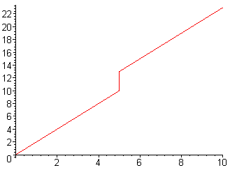
Illustration 1: Example of discontinuity
A Gentle Introduction to Continuity and Limits
Determining the definition for continuity was a major accomplishment of nineteenth century mathematics. The compactness of the definition belies the effort expended in arriving at it. The French mathematician Augustin Cauchy is credited for the delta and epsilon definition found in calculus courses.
I can remember being bewildered the first time I saw the definition of continuity. In what follows I am going to go through a series of steps to show how the definition of continuity could be arrived at by starting with our intuitive concept of continuity and how this reasoning leads to the idea of limits.
In the world that we perceive everything appears to be continuous. The temperature cannot go from 0 to 20 degrees without passing all the places in between. The most common functions are combinations of polynomial, trigonometric and logarithmic functions, and are also continuous. To understand continuity it helps to start with an example of discontinuity. Consider the function below, defined as:
y=2x, 0
< x < 5
2x+3, x
≥5
Illustration
1: Example of discontinuity
We feel that this function is okay except at x=5, where the function suddenly jumps from 10 to 13. We will therefore define continuity at a point and we will define it in such a way as to ensure that the values of f(x) would not be allowed to suddenly jump from f(x) = 10 just before x=5 to f(x) = 13 at x=5. We cannot of course talk about the value of x “just before 5.” What we can do is to talk about values of f(x) on small intervals of x containing 5. We would say that for sufficiently small intervals (a, b) containing 5, the range of values of f(x) on (a, b) is (f(a), f(b)), that is the function will contain all values between f(a) and f(b). By sufficiently small we mean that we can find a δ > 0 such that a and b are within δ of 5, that is in this case a < 5 – δ and 5 < b < 5 + δ.
Definition 1 – A function f(x) is continuous at x = c if we can find a δ > 0 such that for a < c - δ and c < b < c + δ the range of values of f(x) on the interval (a, b) is (f(a), f(b)).
Let us see how this definition applies to the above example. Suppose we choose δ = 0.1. What values of f(x) are taken for x in (4.9, 5.1)? The values of f(x) will be (9.8, 10) and [13, 13.2). The values for f(x) in [10, 13) will be missing no matter how small we make δ, so the function is not continuous at x=5.
So far the definition agrees with our intuition. Let us test it further. There are two types of problem that we can encounter. The definition may include something that we feel should not be included or it may not include something that we feel should be included.
Consider the following function:
y = sin(1/x), x
≠
0
0, x = 0
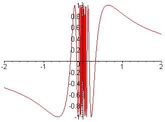
Illustration
2: sin(1/x)
For
large |x|, sin(1/x) will approach sin(0) = 0 and is therefore
asymptotic to the x axis. For small |x|, 1/x goes to infinity and so
the function will oscillate wildly between the extreme values of -1
and 1.
Is this function continuous at x=0? By definition 1 it would be. For any interval -δ < x < δ where δ > 0, f(x) will include all values from -1 to 1 and so will definitely include all values between f(-δ) and f(δ), infinitely many times. Suppose we had defined f(0) to be 7/8 or –1/4 or any other value from -1 to 1. By our definition the function would still be continuous. This does not seem right. Our definition is too inclusive.
The problem seems to be that we are permitting too many oscillations. Let us change the definition to disallow any oscillation. We will not allow the function to bounce up and down. We will have to be able to choose intervals of x sufficiently narrowly so that f(x) will be either steadily increasing or decreasing on the interval. A steadily increasing function satisfies the condition that for x < y, f(x) ≤ f(y) and a steadily decreasing function satisfies the condition that for x < y, f(x) ≥ f(y) where in each case x or y are any two values in the interval. A function that is either steadily increasing or decreasing is called monotonic.
Definition 2 – A function f(x) is continuous at x=c if we can find a δ > 0 such that for a < c - δ and c < b < c + δ the range of values of f(x) on the interval (a, b) is (f(a), f(b)) and f(x) is monotonic on (a,b).
Before deciding on how well this definition covers what we feel should be continuity, let us take a closer look at a typical case covered by definition 2.
Consider f(x) = x2 near x = 2. Because f(x) is monotonically increasing near x=2, x2 keeps getting closer to 4 as x gets closer to 2. Suppose we wanted to stay within 0.5 of 4, so we require that 3.5 ≤ f(x) ≤ 4.5. We simply take the square roots of 3.5 and 4.5 to get, to two decimal places, x = 1.87 and x = 2.12. As long as x is in (1.87, 2.12), f(x) will be within .05 of 4. Notice that 2 – 1.87 = 0.13 and 2.12 – 2 = 0.12. If we chose 1.88 instead of 1.87 as the lower bound we would still be within 0.5 of 4, but now because 2 – 1.88 and 2.12 - 2 both equal .12, we could say, more compactly, that |f(x) – 4| < 0.5 whenever |x – 2| < 0.12. This of course leads us to the delta/epsilon definition of continuity.
Definition 3 – A function f(x) is continuous at x=c if for any ε > 0, δ > 0 can be chosen such that |f(x) – f(c)| < ε whenever |x – c| < δ .
What is different about definition 3 is that instead of looking at values covered in intervals surrounding c, it requires that the values of f(x) have to zero in on the value of f(c) as the size of the interval shrinks.
How does definition 3 compare to definitions 1 and 2? Firstly, we will show that definition 2 is too restrictive.
Let us modify sin(1/x) by multiplying it by x to get:
f(x) = x
×sin(1/x),
x ≠ 0,
0, x =0
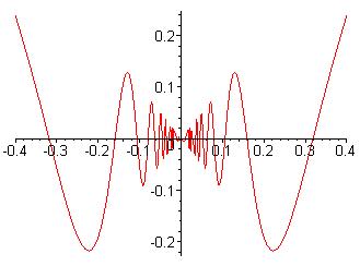
Illustration
3: x × sin(1/x)
For large values of x, f(x) will
asymptotically approach y = 1, because x
×sin(1/x) = sin(1/x) / (1/x) and limit of sin(u)/u goes to 1
as
u goes to zero.
For small values of x, f(x) will still oscillate wildly, but the size of the oscillations will keep getting smaller. Since -1 ≤ sin(1/x) ≤ 1, |x ×sin(1/x) | ≤ x and we can restrict the value of f(x) by restricting the value of x. We can therefore force |f(x) – 0| < ε provided that |x – 0| < ε . By definition 3, taking δ = ε, f(x) is continuous at x = 0. This agrees with our intuition that the function should be continuous. The function would not be continuous by definition 2, because it is not possible to choose an interval around 0 where f(x) does not oscillate.
Now let us compare definition 3 with definition 1. Definition 3, unlike definition 1, says that the sin(1/x) function defined previously is not continuous at x = 0. Suppose that we choose ε = 0.1. We want to keep f(x) between -0.1 and 0.1. No matter how small we choose δ, f(x) will keep fluctuating between -1 and 1 for x in (-δ, δ), and so is not continuous at x=0.
To summarize, we used our intuition to define continuity at a point in terms of not skipping any values of f(x), but were led to the epsilon/delta criterion.
Arriving At The Definition
Sometimes it is the oddball cases that allow us to arrive at a definition. What is crucial about x ×sin(1/x) is that the oscillations keep getting smaller as we approach x=0. Imagine two people standing in a hallway trying to catch a puppy. They slowly move toward each other, so the movement of the puppy becomes more restricted. It is this idea of restricted oscillation that forms the basis of the defintion of continuity.
Limits
We will use the concept of limit to define continuity. We notice that the function x ×sin(1/x) closes in on y=0. In a sense, we can say that 0 is the value that the function "ought to have" at x=0.
We call the value that the function “ought to have” the limit of the function. We will first define what we mean by a function f(x) having a limit L at x=c. We will then be able to define continuity for f(x) at x=c by requiring f(x) to have a limit L at x=c and also requiring that f(c)=L.
Informally, a function f(x) has a limit L at x=c if we can restrict the osicillations of f(x) to be arbitrarily close to L by choosing x sufficiently close to x-c.
Definition of Limit - A function f(x) has a limit L at x=c if for any ε > 0, δ > 0 can be chosen such that |f(x) – L| < ε whenever |x – c| < δ .
Using the definition of limit we can replace definition 3 with the following definition of continuity:
Definition
of continuity at a point
– A
function f(x) is continuous at a point x=c if:
1. The function has
a limit L at x=c
2. f(c)= L
If we took our function f(x)=x×sin(1/x) and defined f(0) = 3, this function would still have a limit of 0 for x=0 but it would be discontinuous at x=0 because f(0) would not be equal to the limit of 0. The function sin(1/x) is of necessity discontinuous at x=0 for any value of f(0) because there is no limit at x=0.
For the concept of limit to have any sense it must be true that there is at most one limit for f(x) at x=c. It is not difficult to visualize why this follows from the definition of limit. To better see this let us work with specific numerical values. Suppose there is some function f(x) that has two limits, L1=30 and L2=40 at x=7. We know from the definition of function that there is a single value of f(7). An informal way of putting this is to say that the function can be in only one place at a time. We want to extend this idea by showing that a continuous function can only be arbitrarily close to at most one place at a time.
The distance between our two limits 30 and 40 is 40 – 30 = 10. In the definition of limit let us take ε = 5 for both limits and let us suppose that δ1 = 0.1 and δ2=0.2. What this means is that |f(x) – 30| < 5 when |x – 7| < 0.1 and |f(x) – 40| < 5 when |x – 7| < 0.2. Since the values of x such that |x – 7| < 0.1 are included in the values of x such that |x – 7| < 0.2 it follows that for |x – 7| < 0.1, |f(x) -30| <5 and |f(x) – 40| < 5. For 6.9 < x < 7.1 we have 25 < f(x) < 35 and 35 < f(x) < 45. The two regions do not overlap so f(x) cannot be in both of them at the same time. We are led to a contradiction, so our assumption of the existence of two limits is incorrect.
Rather
than talking about non-overlapping regions in the above proof, there
is a useful inequality that can be used:
|a + b| ≤ |a| + |b|.
It should be obvious that equality will only hold when a and b are
either both positive or both negative.
To
see
how to apply this inequality in the above argument let us start from
the point at the end where we found that
for |x – 7| <
0.1, |f(x) -30| <5 and |f(x) – 40| < 5. Express
the
distance from 30 to 40 as the sum of the distance from 30 to f(x) and
the distance from f(x) to 40.
For |x – 7| < 0.1,
10=|40 – 30| = |(40 – f(x)) + (f(x) –
30)| ≤
|f(x) – 40| + |f(x) – 30| < 5 + 5 =10. This
leads to
10<10, which is a contradiction.
I think it is worthwhile to see how all this is formalized into a general proof.
Theorem
– A function f(x) can have at most one limit at x=c.
Proof
- Suppose f(x) has two limits L1 and
L2.
Using
|L1
–
L2
|/2
for ε in the
definition of limit for both L1
and L2
we know
that there is some value δ1
such that |f(x) –
L1 |
< |L1 –
L2 |/2
whenever |x -c| < δ1
and there is some value
δ2
such that |f(x) – L2
| < |L1
–
L2 |/2
whenever |x -c| < δ2.
Let δ be the minimum of δ1 and δ2 . Then |f(x) – L1 | < |L1 – L2 |/2 and |f(x) – L2| < |L1 – L2 |/2 whenever |x – c|<δ. To get our contradiction we use the fact that |L1 – L2 | = |(L1 – f(x)) + (f(x) – L2 )| ≤ |f(x) – L1 | + |f(x) – L2 | < |L1 – L2 |/2 + |L1 – L2 |/2 for |x-c| < δ. This gives |L1 – L2| < |L1 – L2| which is a contradiction so that there can be at most one limit and our theorem is proved.